How to interpret the terminal region of the Gradient Boosting Machine
Including related examples, math, and code
Gradient Boosting Machines are among the popular machine learning models these days, as they can find any relationship between the dependant and independent variables by applying binary rules in their base learner which are the decision tree regressors (mostly). For this matter, you can apply well-known libraries including XGBoost, CATBoost, BoostedTrees, etc to build a robust Gradient Boosting model on your dataset.
In this review, we will learn more about the details of the Base learner, and interpret the final predicted values of each base learner.
Gradient Boosting Model
Gradient Boosting Model is one of the ensemble machine learning models that use multiple weak learners to achieve better performance.
For classification and regression problems, the Gradient Boosting Machines include the Regressor Tree as the weak learner. The idea is to predict the residual of the previous boosting step by the weak learners and use the least square to optimize the decision tree at each epoch.
To optimize each tree, it considers different impurity criteria including Gini, least square, etc. You can find more about the tree impurity criteria, here.
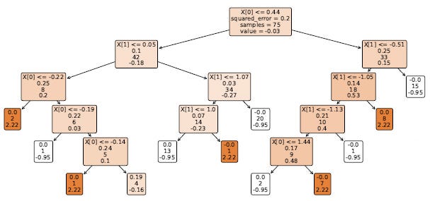
After building the decision tree regressors, we will have the final prediction of the terminal nodes of the tree. (Let’s call them the leaves values) (Highlighted with warmer color in the figure)

Building the regression tree will continue until the last number tree, which we already have defined it the model parameter. Or, if the model has the early stop, it determines the stoping criterion by itself. At each epoch, by having the learning rate and predicted values by the trees, we advance the prediction at the current step.
Decision Tree Regressor
We studied an overview of the Gradient Boosting Machine approach and the overall training procedure. As the study focus is the tree’s final prediction value, we skip other parts (Impurity function, shrinkage rate, loss function, residual, etc.) and jump into the tree leaves’ values.
We knew that at each iteration, we have k trees for each class in which each of them predicts the previous residual and returns a continuous value. Therefore, at the leaves, we have the prediction as a scaler value.
One approach to achieve the values of the leaves values (not the children’s values) is to train the gradient Boosting model from the Sklearn library and use the following method to return the leaves’ values.
Here we will have the leaves values of each class and tree.
By having the results and values, you may want to interpret them, and one way would be plotting the values on the x-axis of each node.

To have a smoother plot, you can apply a B-spline function on your curve and consider the y-axis (leaves values) as the control points of the B-Spline function. The most important parameter in the B-Spline function is the value of the degree. Degree three will return the cubic degree function.

In the following, I included the function which returns the smoothed curve of the leaves values.
In this function, the data would be the output of the terminal_leaves(model, tree, class_).
Conclusion
The gradient boosting machines and the training approach is described in this study. We have reviewed the decision regressor tree and its training as the weak learner of the ensemble model. The goal of this study was to interpret the performance of the decision tree regressor. As there are many studies about the tree’s performance, in this article, we introduced a new approach to interpreting the tree with its terminal values.
The related codes to apply the model, and return the model leaves are added with the related functions.
