Analysis of the performance of the ensemble model for a multi-output regression problem
A regression problem in general refers to the tasks with real or continuous variables as the target. There are many popular machine learning models that are able to be applied to this problem, including the linear regression model.
In the following article, I review the examples of the regression problems, introduce two regressor models, apply the regressor models to multi-output regression tasks, review the results of each model and introduce different metrics to evaluate the model’s performances.
Regression Dataset
The regression tasks include problems with continuous values for the target variable. The regression tasks can be found in the well-known repositories, such as UCI, and Kaggle, or can be generated as a synthetic regression dataset with a specific instance, features, and bias.
One method to generate a random set of a regression problem is the make_regression method from Sklearn.
from sklearn.datasets import make_regression
make_regression(n_samples=100, n_features=100)
In this study, I consider the Energy dataset with two different targets with 768 instances, 8 features, and 2 outputs.
Machine Learning models
A standard assignment in different machine learning models is to build a non-parametric regression or classification model from the related dataset. The primary concept of boosting approach is to add sequentially a new weak learner to the ensemble.
I apply two ensemble models from the Gradient Boosting Machines category for this part. The first one is the current gradient model (GB), and the latter is the XGBoost derivative, the LightGBM.
GBM
The gradient boosting machines is based on Friedman’s gradient-descent boosting methods [1]. Gradient boosting is an ensemble machine learning model for both regression and classification. The gradient model is a linear ensemble of a series of weak models that are sequentially created. The GBM minimizes the expected loss function over the response variable. One loss function for the regression could be the least-squares that draws a line between the prediction and real values and tries to minimize the vertical distance. The following code will apply the GBM regression.
from sklearn.ensemble import GradientBoostingRegressor
gbm = GradientBoostingRegressor()
The default parameters of the models are as follows;
{'alpha': 0.9, 'ccp_alpha': 0.0, 'criterion': 'friedman_mse', 'init': None, 'learning_rate': 0.1, 'loss': 'squared_error', 'max_depth': 3, 'max_features': None, 'max_leaf_nodes': None, 'min_impurity_decrease': 0.0, 'min_samples_leaf': 1, 'min_samples_split': 2, 'min_weight_fraction_leaf': 0.0, 'n_estimators': 100, 'n_iter_no_change': None, 'random_state': None, 'subsample': 1.0, 'tol': 0.0001, 'validation_fraction': 0.1, 'verbose': 0, 'warm_start': False}I talked about each different parameter in my previous reviews.
LightGBM
While Gradient Boosting tracks negative gradients to optimize the loss function, XGBoost uses Taylor expansion to calculate the value of the loss function for different base learners.
The loss function, regularization term, derivation of the loss, and solution approach for the optimization problem are different from the previous
model.The objective of LightGBM is based on the second-order Taylor expansion of the loss. The same as the XGBoost.
One of the advantages of the lightGBM is that it uses a different approach for splitting the tree node. For this matter, it applies a histogram binarizing strategy that stores continuous features in discrete bins
Training the model
Note that both models natively work for single output regression tasks, therefore, we can not apply them to Energy dataset. For the purpose of this study, I trained separately both models, two times for each target of the Energy dataset.
ight_gbm = HistGradientBoostingRegressor()    pred_light = np.zeros_like(y)
    for i in range(y.shape[1]):
        light_gbm.fit(X, y[:, i])
        pred_light[:, i] = light_gbm.predict(X)
After the training procedure, I stored the predicted values in 2-D arrays for further investigations.
Evaluation
There are various approaches to evaluate the regression tasks. For instance, the standard metric including R2 score, RMSE, MSE, and MAE could be applied.
Scatter plot
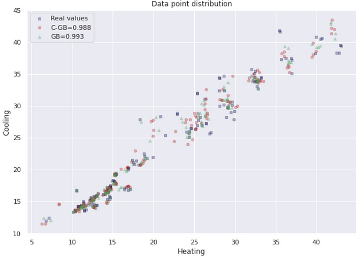
In the following, I applied a scatter plot to review the distribution of the predicted values for each model and real values.
The axes of the plot represent two targets of the regression dataset, which are the Heating and Cooling variables.

Another approach would be, scattering the predicted values and real values on a plot for each target and model. Therefore, the X-axis presents the real values and the y-axis indicates the predicted values. Due to the big amount of data points, the scatter plot could not interpret easily, hence, it can be applied to the hexbin plot, in which each hexagon shows the bins of the data point. We are looking for a linear regression which would be a thinner diagonal.

Moreover, the RMSE for each target is calculated and indicated on the plot. Both RMSE and scatter reveal the better performance of the GB model.
Conclusion
In this review, we talked about the single output and multi-output regression tasks and introduced the Energy Dataset. Likewise, the related Ensemble models were introduced and examples of the code were included. Finally, two new metrics were introduced and the results were interpreted and compared.
References
[1] Friedman, J. (2001). Greedy boosting approximation: a gradient boosting machine. Ann. Stat. 29, 1189–1232. doi: 10.1214/aos/1013203451.
[2] Ke, Guolin, et al. “Lightgbm: A highly efficient gradient boosting decision tree.” Advances in neural information processing systems 30 (2017): 3146–3154.
